The GraphQL ecosystem has mature tools for browsing GraphQL schemas in a web browser (e.g. GraphiQL) or GUI app (e.g. altair). These tools are great, but in terms of flexibility and composability, nothing beats the command line for me. While working on the server-side of a complex GraphQL service, I repeatedly found myself wanting a CLI to help make sense of it. Something that I could run without leaving the terminal environment, and pipe to other commands I use frequently (grep, awk, sort, jq, etc.).
There are tools like graphql-cli out there, but I found the initial setup process for graphql-cli to be somewhat overwrought. This isn’t to say that graphql-cli is bad - it looks like a well-thought-out and higly extensible tool, but I think my philosophy on tool design is different from that of the authors: when the entrypoint to a CLI tool is a configuration wizard, I know that it’s not for me.
So, I wrote my own CLI tool for working with GraphQL schemas: gquil.
The rest of this post walks through a few examples of how to use gquil, using the GitHub GraphQL API to demonstrate.
GitHub has some nice documentation on how to obtain the full GraphQL schema for their API. They offer several options for doing so, but if you want to obtain the schema in GraphQL SDL form, you can do something like this:
This will yield a ~60k-line document in the GraphQL schema language (aka ‘GraphQL SDL’), describing all of the types, fields, interfaces, enums, etc. that comprise GitHub’s GraphQL API.
GraphQL schemas can also be queried using GraphQL itself, via something called the introspection schema. Introspection query responses can be serialized to JSON, leading to an alternative mechanism for representing the schema.
However, there are a few drawbacks to this ‘introspection JSON’ format:
Since GraphQL uses client-specified response shapes, there isn’t really a single JSON schema that describes the exact shape of ‘introspection JSON’ in all cases. What you get back depends on the introspection query you write! The reference GraphQL JS implementation does export an introspectionQueryvariable, but it’s not part of the official GraphQL spec, which describes the introspection schema, but leaves queries against it up to you.
The introspection schema omits information about the application sites of custom directives within a schema (Apollo calls directives applied to schemas ‘schema directives’ to differentiate them from schemas applied to operations). This directive information is sometimes of great interest to schema maintainers.
It’s quite verbose compared to the SDL format.
The JSON representation of the introspection schema uses variable levels of nesting to represent things like wrapping types (lists and non-nullable types). This aligns with GraphQL’s hierarchical nature, but makes processing of it with tools like jq harder than it should be (more on this later).
GraphQL servers almost universally support the introspection schema (though public access to it may be disabled for security reasons), but not every GraphQL service necessarily has a GraphQL SDL representation of its schema. This is especially true of ‘code first’ GraphQL servers, where the schema is defined programatically in the native programming language of the server, rather than being specified in GraphQL SDL to begin with.
For these reasons, gquil makes it easy to generate a GraphQL SDL representation of a schema from an introspection endpoint. Here’s an example of how to do this with the GitHub API:
… where TOKEN is a GitHub auth token. The -H / --header flag works similarly curl’s, allowing you to pass in any headers that might be needed to authenticate against the server.
You can also see the exact query being executed against the server like this:
… or by adding the --trace flag to an invocation of introspection generate-sdl, which will emit details of the outbound request and inbound response to stderr.
You can limit the set of returned fields to only those defined on a specific type:
❯ gquil ls fields --on-type Actor github.graphql
Actor.avatarUrl: URI!
Actor.login: String!
Actor.resourcePath: URI!
Actor.url: URI!
Sometimes you want to see all of the ways in which a particular type is used within a schema. For that, you can use --of-type to only return fields which are of a specified type (or a wrapped variant of that type):
❯ gquil ls fields --of-type User github.graphql
AddEnterpriseOrganizationMemberPayload.users: [User!]
AddedToMergeQueueEvent.enqueuer: User
AssignedEvent.user: User
... snip ...
Note how AddEnterpriseOrganizationMemberPayload.users is returned, even though its type is [User!] rather than User.
Sometimes, you want to see all fields which might possibly return a given type. For example, in the GitHub API, there’s an interface called Actor, which is implemented by multiple types, including User. If we ask for all fields of type User (or a wrapped type thereof), we see that there are 148 of them:
❯ gquil ls fields --of-type User github.graphql | wc -l
     148
… but what about fields which are typed as Actor instead? These fields might possibly return an instance of User, but are excluded from the above listing. To include them, we can use --returning-type instead, which accounts for interface and union types:
❯ gquil ls fields --returning-type User github.graphql | wc -l
     369
We can also filter fields by name using the --named flag. Sometimes, fields are named the same, even though they’re of different types. For example, in the GitHub API, we can see that fields named user are usually typed as User (or User!), but there is one case where a field of this name is typed as Actor instead!
❯ gquil ls fields --named user github.graphql \
  | awk '{ print $2 }' \
  | sort \
  | uniq -c
   1 Actor
  74 User
  12 User!
Let’s find out which one that is:
❯ gquil ls fields --named user --of-type Actor github.graphql
SavedReply.user: Actor
GraphQL also supports custom directives that can be attached to various parts of a schema. Vendors like Apollo use these directives heavily for supporting federation. You can list all custom directives within a schema too, like this:
❯ gquil ls directives github.graphql
@possibleTypes(abstractType: String, concreteTypes: [String!]!) on INPUT_FIELD_DEFINITION
@preview(toggledBy: String!) on ARGUMENT_DEFINITION | ENUM | ENUM_VALUE | FIELD_DEFINITION | INPUT_FIELD_DEFINITION | INPUT_OBJECT | INTERFACE | OBJECT | SCALAR | UNION
@requiredCapabilities(requiredCapabilities: [String!]) on ARGUMENT_DEFINITION | ENUM | ENUM_VALUE | FIELD_DEFINITION | INPUT_FIELD_DEFINITION | INPUT_OBJECT | INTERFACE | OBJECT | SCALAR | UNION
All of the ls subcommands described above default to a compact, line-based output format suitable for use with grep, awk, sort, etc. Sometimes, you want more information about each listed item, and more flexibility in terms of how to process the list. For those cases, all ls subcommands also support a JSON output format via the --json flag.
Returning to an example from above, let’s say we wanted to find the types of all fields which might possibly return a value of type User. Previously, we had this command to find all fields which might return a User:
❯ gquil ls fields --returning-type User github.graphql
Adding --json to that incantation, we get output like this:
❯ gquil ls fields --returning-type User --json github.graphql
[
  {
    "description": "The subject",
    "name": "AddCommentPayload.subject",
    "type": {
      "kind": "INTERFACE",
      "name": "Node"
    },
    "typeName": "Node",
    "underlyingTypeName": "Node"
  },
  {
    "description": "The users who were added to the organization.",
    "name": "AddEnterpriseOrganizationMemberPayload.users",
    "type": {
      "kind": "LIST",
      "ofType": {
        "kind": "NON_NULL",
        "ofType": {
          "kind": "OBJECT",
          "name": "User"
        }
      }
    },
    "typeName": "[User!]",
    "underlyingTypeName": "User"
  },
... snip ...
We can use this output in combination with a generic JSON processing tool like jq to answer our question as follows:
The JSON output format for gquil is inspired by GraphQL’s introspection schema, but differs in a few important ways:
When you ask for the type of a field in the introspection schema, you get back a full __Type object, allowing you to recursively traverse the type graph. This makese sense if you’re writing GraphQL queries against a schema, but is difficult to shoehorn into a model where you’re emitting JSON in a standardized shape (where do you stop the recursion?). For this reason, references to other named types in the JSON output format of gquil are just strings which name the referred-to type.
The JSON output format for gquil includes information about directives that have been applied at various places within the schema (this information is mostly omitted from the introspection schema, with a few special-case exceptions for built-in directives like @deprecated). Sometimes, information about the set of applied directives is useful for filtering and processing schema elements (e.g. when you want to find all fields that have a specific directive applied to them).
As a convenience, the gquil JSON output format adds an underlyingTypeName field to its representation of GraphQL fields, which contains the ‘unwrapped’ type name of the field. For example, a field of type [String!] would have an underlyingTypeName of String. There’s also a typeName field, which contains the string representation of the field’s type, with any wrapping decorations (e.g. [String!] for the previous example).
Sometimes it’s interesting to be able to answer questions like “what is the full set of types needed to represent anything that might possibly be returned by this field?”. This might come up, for example, when you’re considering extracting parts of your GraphQL schema into a subgraph.
For example, here’s how you could list all fields which are reachable if you start from the Query.license entrypoint within the GitHub schema:
This style of filtering can be applied to both ls fields and ls types:
❯ gquil ls types --from Query.license github.graphql
OBJECT License
OBJECT LicenseRule
OBJECT Query
SCALAR URI
You can also specify the --from flag multiple times in order to use multiple starting points. For example, to show all types reachable from Query.licenseorQuery.codeOfConduct:
❯ gquil ls types --from Query.license --from Query.codeOfConduct github.graphql
OBJECT CodeOfConduct
OBJECT License
OBJECT LicenseRule
OBJECT Query
SCALAR URI
Finally, you can use the --depth flag with --from in order to limit the depth of the traversal from the root. A depth of 1 means only the referred to object itself:
❯ gquil ls types --from VerifiableDomainOwner --depth 1 github.graphql
UNION VerifiableDomainOwner
Increasing the value of the --depth parameter includes more distantly-related types & fields:
❯ gquil ls types --from VerifiableDomainOwner --depth 2 github.graphql
OBJECT Enterprise
OBJECT Organization
UNION VerifiableDomainOwner

❯ gquil ls types --from VerifiableDomainOwner --depth 3 github.graphql | wc -l
      82
Finally, the good stuff. Producing lists of schema elements in line-delimited or JSON format is nice, but sometimes, you need a picture. For that, there’s gquil viz, which can emit visualizations of your GraphQL schema in GraphViz DOT format.
First, if you’ve never used GraphViz, run, don’t walk to your local package manager:
❯ brew install graphviz
This will give you (among other things) a tool called dot, which can turn simple textual representations of graphs into pretty pictures. You can now use this tool in combination with gquil plus your GraphQL schema.
A note of caution: big schemas = big visualizations #
If you have a non-trivial GraphQL schema, and just try to run it through gquil viz and then render the resulting graph, it is very likely to yield an unintelligible tangle that takes forever to render.
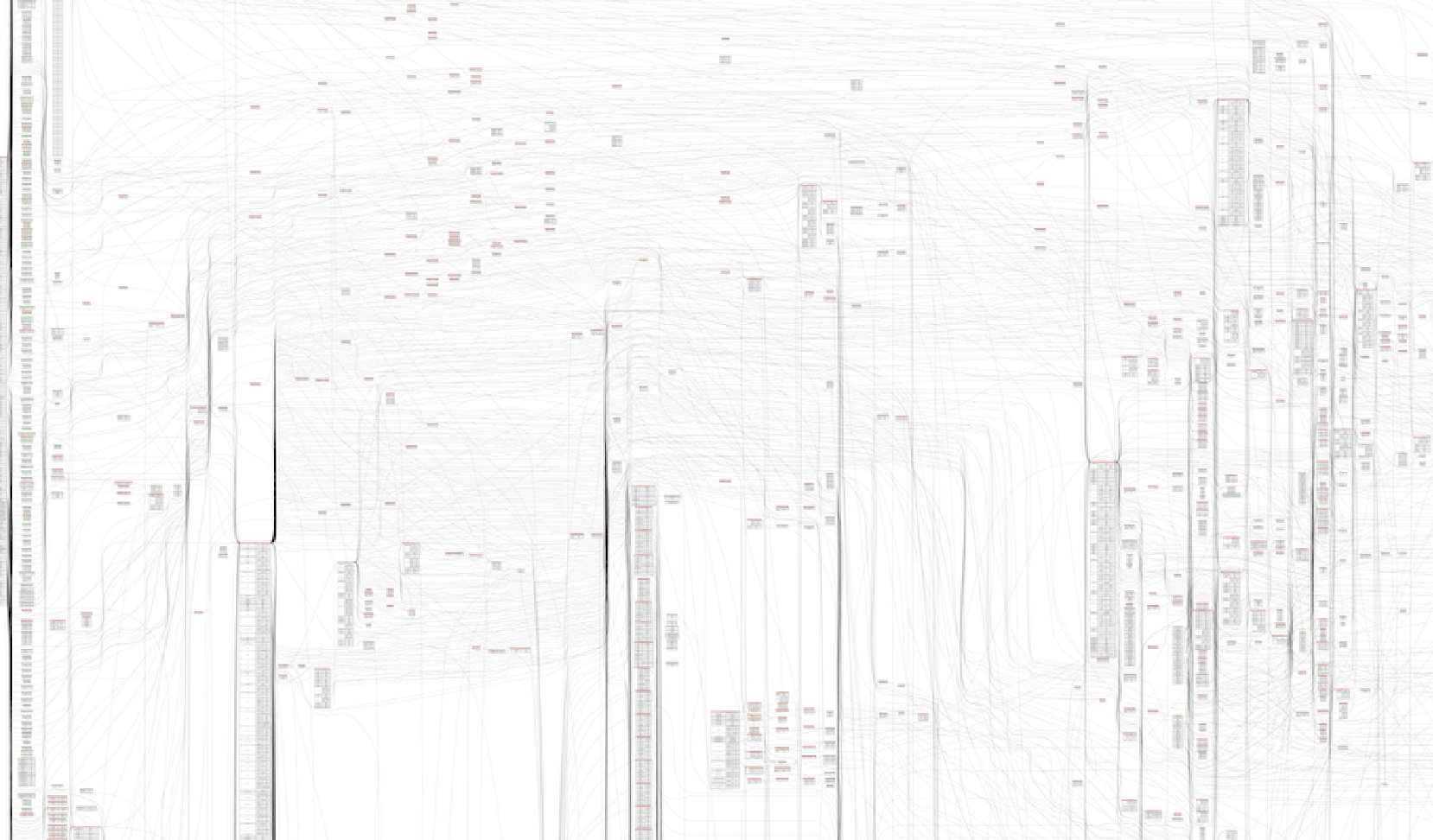
For example, here’s how the GitHub schema looks when rendered by gquil with GraphViz:
❯ time gquil viz github.graphql | dot -Tpng >out.png
dot: graph is too large for cairo-renderer bitmaps. Scaling by 0.361918 to fit
gquil viz github.graphql  0.13s user 0.03s system 118% cpu 0.130 total
dot -Tpng > out.png  305.79s user 3.88s system 98% cpu 5:13.85 total
After about 5 minutes, this command produces an 88 MB(!) PNG file, which you can get the flavor of from the cropped section below:
To get a useful visualizaiton, you need to get more specific about what you want to see. To support this, the viz subcommand supports the same --from and --depth flags described above in the section on listing schema elements.
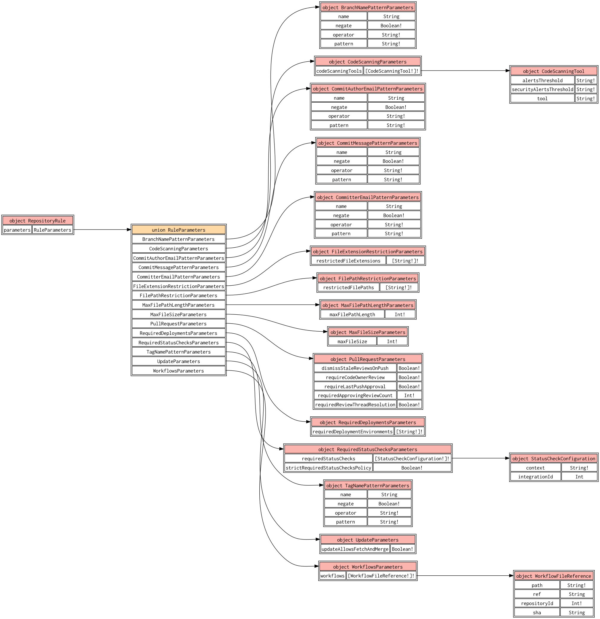
For example, let’s say I wanted to visualize the possible values for the RepositoryRule.parameters field:
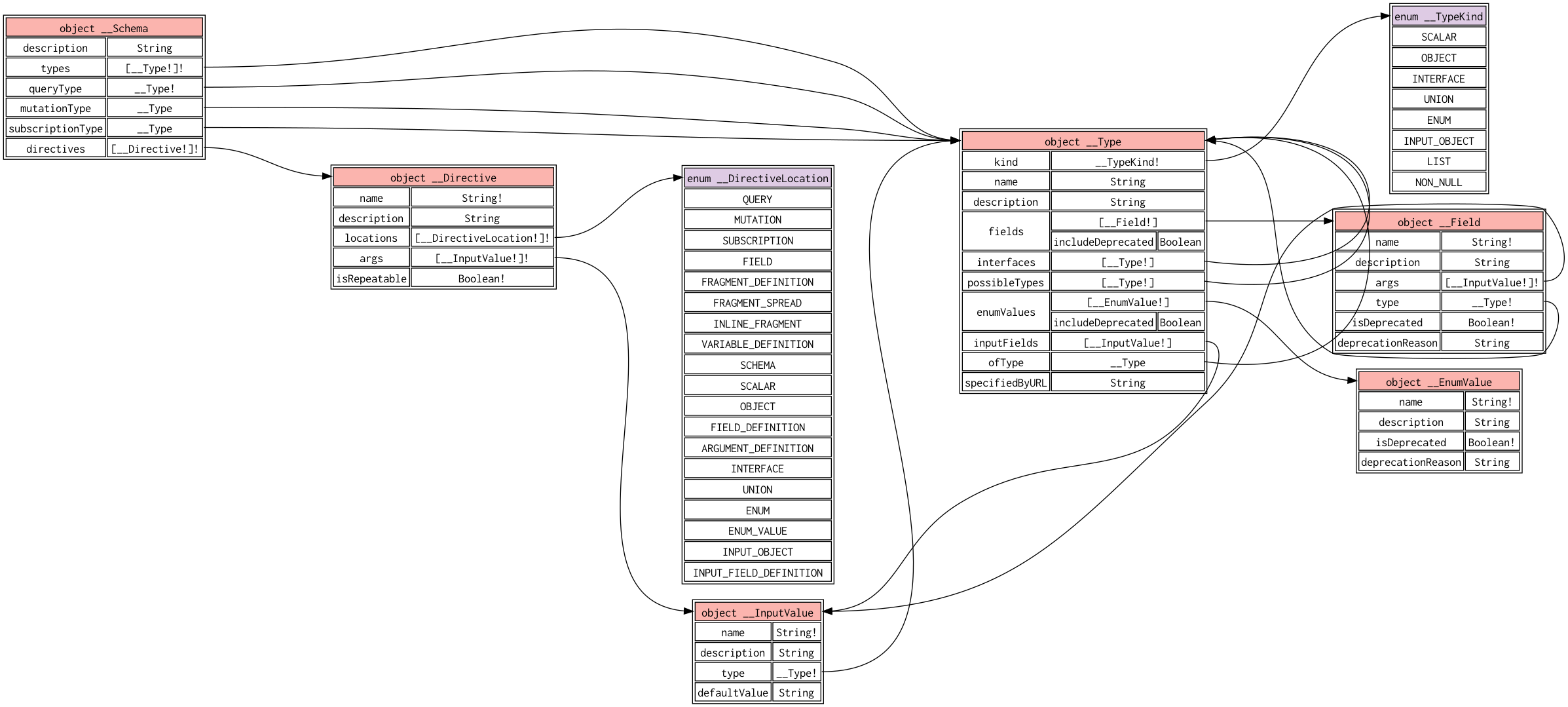
For a fun trick, here’s a visualization of the built-in introspection schema defined in the GraphQL spec (in this example, we’re feeding an empty schema into gquil viz on stdin, and using the --include-builtins flag to force it to render built-in types):
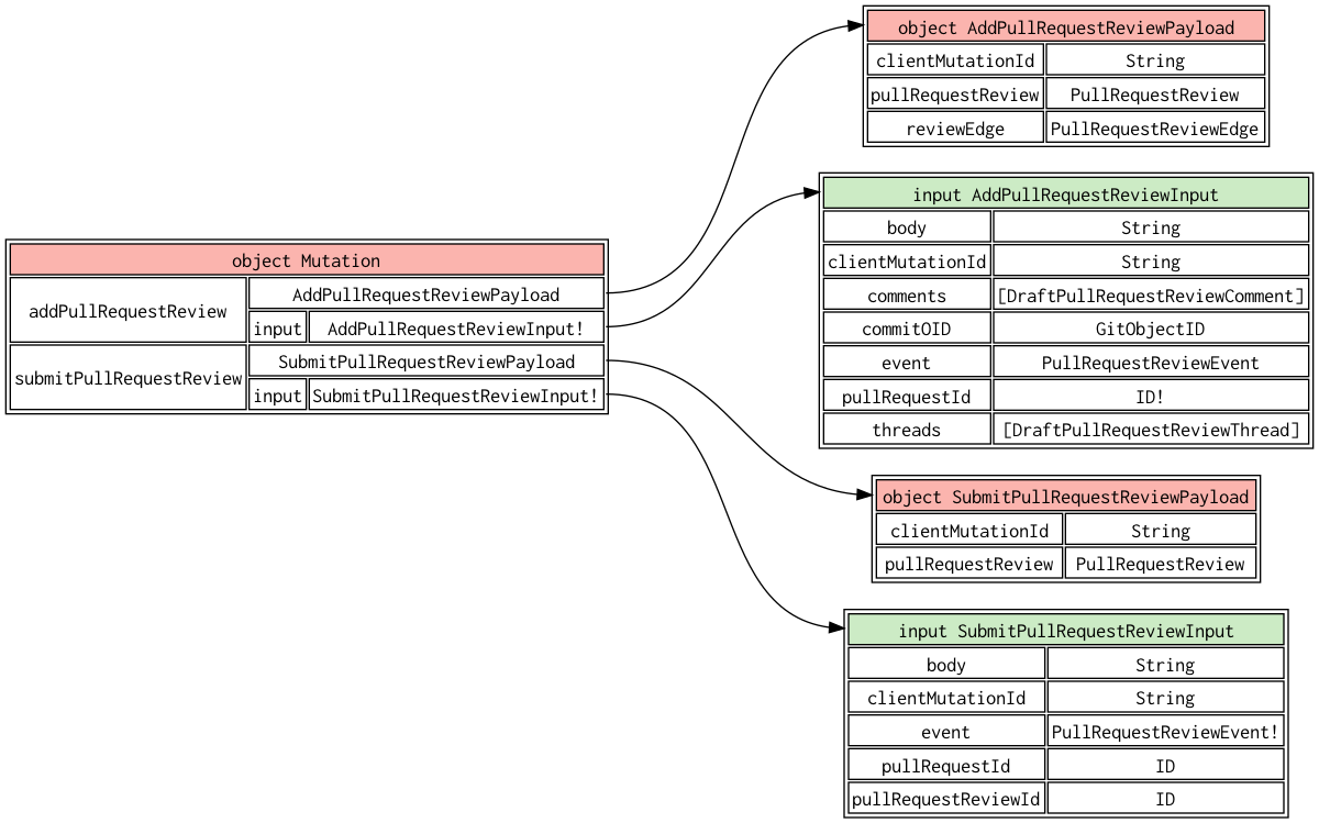
You can of course use the --depth flag to limit the depth of traversal here too, and specify --from multiple times to pull in multiple root fields or types:
I wrote gquil originally for myself, but I’m curious to hear how it has worked (or not worked!) for you! If you happen to give it a try, I’d love to hear any feedback you have about the tool and how it could be better or more useful. See the contributing guide for details.
There are some things that almost everyone is familiar with, but which relatively few people understand deeply. You might go your whole life never awakening to your own lack of knowledge on a topic that you deal with in a passing manner daily.
For me, URIs were like this (and still are, to some extent). During a recent work discussion about how to structure internally-used URIs, a co-worker helped me realize this.
RFC 3986 formally defines the structure of a URI, along with related concepts like relative references. If you’ve never tried, it’s worth reading (or at least skimming the table of contents)! I’ll admit to only having tried for the first time a few weeks ago, despite working as a software engineer for the last 15 years.
One of the most surprising things I learned while reading it was that URIs do not need to contain two slashes (//). In order to understand the alternative constructions of URIs that looked different from what was in my head, I spent some time making a railroad diagram from (as subset of) the ABNF definitions in Appendix A of RFC3986. They’re pretty, and you might enjoy them:
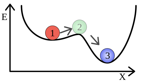
In the physical sciences, there’s a concept called metastability which is an apt metaphor for understanding certain kinds of software engineering failure modes. My grasp of this physics concept is entirely based on Wikipedia’s description, so take this with a grain of salt, but imagine you have a ball sitting in a well, like the red one labelled ‘1’ below:
Undisturbed, it will sit happily. Nudge it a bit and it’ll roll right back into the bottom of the depression on the left and eventually come back to a rest. Nudge it enough, though, and it’ll hit position 2 and then tip down into the deeper well of position 3, from which it’ll be more difficult to dislodge.
Software systems sometimes exhibit behavior like this: small perturbations (a spike in load, an interruption in network availability, a slow disk access) might cause a temporary degradation of service, but generally will resolve without intervention. Sometimes, however, a critical threshold is crossed wherein a feedback loop takes over, holding the system in a bad state until a radical intervention (rebooting, load shedding, etc) is undertaken.
The paper Metastable Failures in Distributed Systems by Bronson, Aghayev, Charapko, and Zhu discusses these kinds of failures in more detail, and provides a succinct definition:
Metastable failures occur in open systems with an uncontrolled source of load where a trigger causes the system to enter a bad state that persists even when the trigger is removed.
The authors stress that it is the feedback loop (the depth of the second well in our ball analogy), rather than the trigger (the nudge) that should rightly be thought of as the ‘cause’ of a metastable failure:
It is common for an outage that involves a metastable failure to be initially blamed on the trigger, but the true root cause is the sustaining effect.
This failure mode might sound rare, but my team at work recently spent some time tracking down a metastable failure state in a very standard looking system: a pool of stateless HTTP servers, each with a database connection pool, which looked something like this:
This system was replacing an older one, but before the replacement we ran an extended load test by mirroring all production traffic from the old system to the new one (silently discarding the results from the new system). In so doing, we encountered a failure mode that only manifested occaisionally, but was catastrophic when it did. The symptoms:
Near 100% CPU utilization on the target database
Application latency pegged at our app-layer timeout (2 seconds)
100% error rate for the application (with all failures being timeouts)
Observed across multiple application instances concurrently
No obvious changes in inbound application throughput or access patterns
Once triggered, the application would remain in this bad state until it was stopped and restarted (scaled to zero and then back up to the target instance count).
Closer examination revealed that the application instances were cycling through database connections at a very high rate. In fact, each request was attempting to establish a new database connection, but timing out before it was able to finish doing so, leaving the connection pools effectively empty.
A failure mode like this can be hard to believe until you’ve successfully triggered it on-demand. While investigating this failure, we relied on a slimmed down test case involving a single application instance and a local database. Running locally, the cost differential between establishing a new DB connection and issuing a query over an existing one was smaller (we did local testing without TLS on the database connection, and without utilizing a database proxy component that was present in production), so it took some finagling to get a suitable reproduction case.
In order to better simulate the cost of new connection establishment, we wrapped a rate limiter around DB connection creation, forcing new connection attempts to block once the threshold rate was exceeded. In reality, the database CPU effectively functioned as this rate limiter. A full TLS handshake takes an appreciable amount of CPU time. Add to that other database-specific CPU work needed to prepare a new connection for use, and you can begin to see how a small number of instances, each with a modest connection pool might saturate the CPU of a database with reconnection attempts.
Simultaneously, my team had been working on ways to induce the issue under production load levels. The initial idea was to consume all available database CPU resources for a brief period of time (long enough for us to trigger application timeouts and thus connection reestablishment). This proved to be more challenging than it might sound (unsurprisingly, most material you’ll find online about consuming database CPU resources is written with the premise that you want to use less not more of them).
The thing that did finally work to trigger this failure mode was to hold an ACCESS EXCLUSIVE lock against a table read by most application requests for a few seconds, like this:
Using this approach, we were able to reliably trigger the failure state, which was critical to building our confidence that we had actually addressed the issue once we implemented a mitigation strategy.
Metastable Failures in Distributed Systems discusses several strategies for dealing with metastable failure states. The one we employed on my team to address this particular problem was a simple circuit breaker around all database interactions.
Our circuit breaker works by keeping a running count of the number of consecutive query failures it has observed, and immediately aborting any database queries for a certain amount of time once a configurable number of failures has been observed. The amount of time queries are disabled for scales exponentially with the number of failures (up to a fixed upper bound), and any successful query resets the failure count back to zero.
The state diagram looks like this:
A circuit breaker breaks the feedback loop: requests that arrive during the period when the circuit breaker is open are immediately aborted, shedding load on the database. The consecutive failure counter ensures that we don’t needlessly open the circuit breaker unless we have strong evidence that the next query is likely to fail.
Without the circuit breaker, we were able to repeatedly trigger a persistent failure state using the locking approach described above. Once the circuit breaker was implemented, the same reproduction steps yielded recovery within seconds after the release of the lock. We’ve not seen any organic recurrences of the issue since the addition of the circuit breaker either.
We can better understand this failure mode using a simplified simulation. I created one using SimPy, a discrete event simulation framework for Python. (Discrete event simulation just means that instead of simulating every ‘tick’ of simulated time, the simulation jumps between discrete events, which may trigger or schedule other events.)
The simulation models a fixed number of application instances, each with a fixed-size database connection pool, all connecting to a single database instance. Requests are randomly distributed amongst instances, and each request involves executing a single database query. The database query consumes a small amount of database CPU time, and simulates network latency between the application and the database by holding the connection from the pool for some additional time.
Requests have a timeout, and if the timeout fires during the execution of the database query, the connection that was being used for that request is marked as dead, and will be refreshed on the next use. The refresh process incurs a higher database CPU cost.
In order to simulate a trigger, the model holds all database CPU resources for a few seconds after an initial delay. A well-behaved system is expected to experience application timeouts during this period, since no other database queries get CPU time to execute. At lower throughput values, this is indeed what happens: the application sees a brief period of timeouts that is similar in duration to the triggering event itself. However, at higher throughputs, the application never recovers from its error state, as repeated timeouts lead to reconnection attempts, which in turn consume database CPU resources, and cause further timeouts.
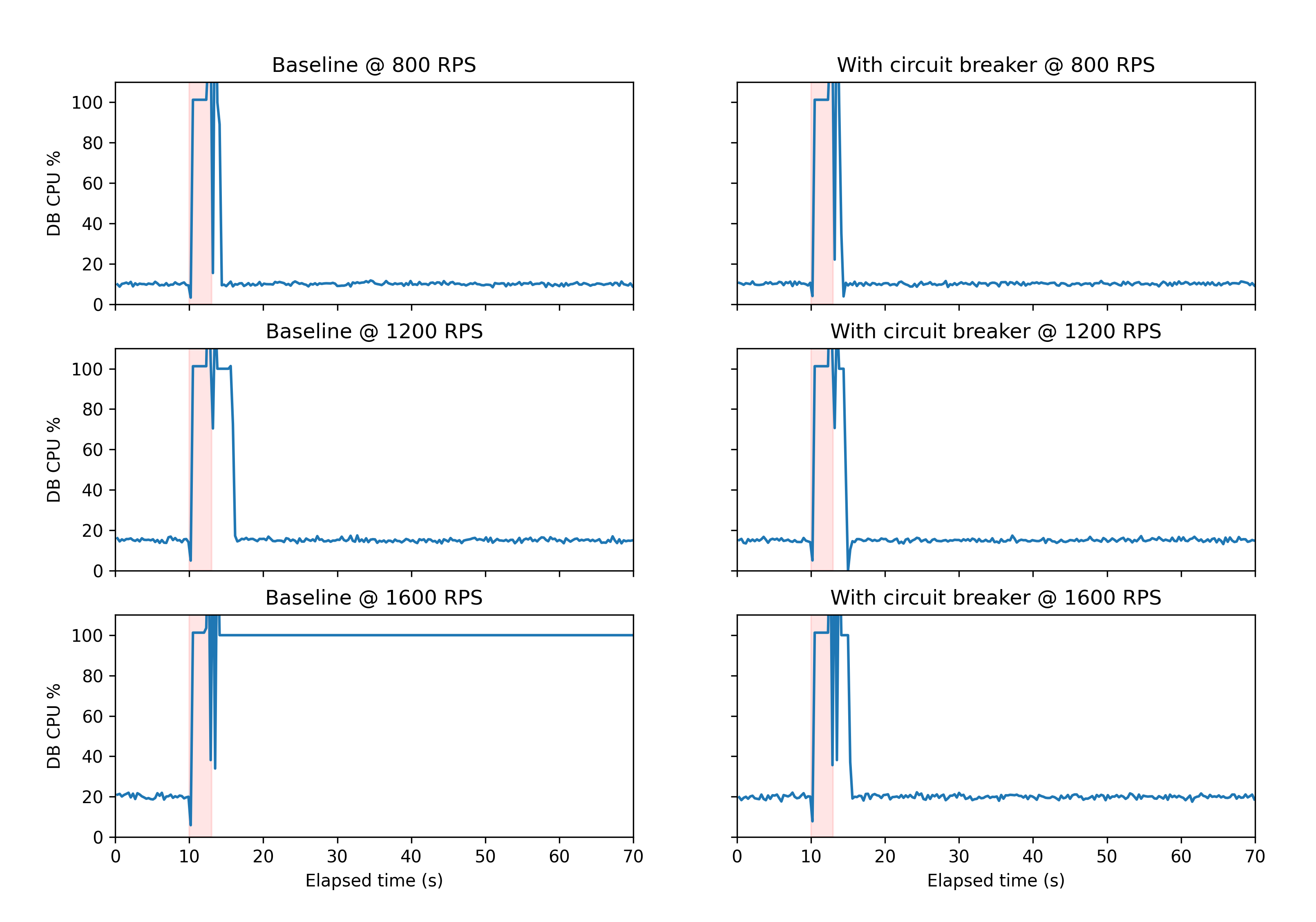
The addition of a circuit breaker to the system allows for recovery from this state. In the charts below, you can see the results of simulating 70 seconds worth of time both without (left column) and with (right column) a circuit breaker.
The y-axis in each chart shows the database CPU utilization, and the x-axis shows time. The pink shading indicates the time during which the database CPU is artificially pinned at 100% usage by the simulation in order to induce the failure mode.
If your system seems to ‘enter a bad state’ under load from which it can’t recover without operator intervention, you too might have a metastable system. They’re not as rare as you might think! Check out the section 3 (‘Approaches to Handling Metastability’) of the paper I linked to previously to get some ideas as to how you might break the feedback loop in your system.
Many thanks to my friend Bill Dirks, who was a sounding board and consistent source of ideas and encouragement during the process of tracking this issue down!
This post was inspired by a Twitter thread by @thingskatedid:
🧵 Make yours and everybody else's lives slightly less terrible by having all your programs print out their internal stuff as pictures; ✨ a thread ✨ pic.twitter.com/NjQ42bXN2E
You should read the whole thread, there are lots of beautiful examples! Her main point is that you should enable your programs to dump their internal state representations visually. Graphviz is a convenient way to do this, since it’s easy to generate and read, and handles the actual rendering for you, but it can feel clunky to repeatedly cycle through the following workflow:
Make code change
Run your program (with flags to dump its internal state in Graphviz form)
Redirect output to a temporary .dot file
Remember the right Graphviz incantation to turn the .dot file into a .png or something (dot -T png in.dot >out.png, FWIW, but it took me years to commit that to memory)
Open the resulting .png in your graphics viewer of choice
Kate talks about how to shorten this feedback cycle in this thread. This is just my distillation of her suggestions.
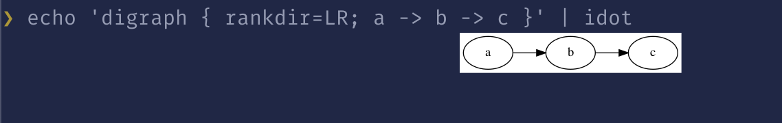
If you use any terminal background color other than white, you’ll find that by default, your graphs don’t look as nice as Kate’s examples:
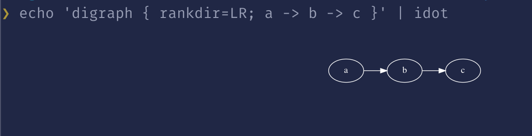
To remove the background colors and make the text, borders, and edges white, you can set a few attributes:
digraph{margin=0.75bgcolor="#ffffff00"color=whitefontcolor=whitenode[color=white,fontcolor=white]edge[color=white]// ... the rest of your graph ...}
If you don’t want to bother with setting these in every chunk of dot you produce, you can modify your idot alias to set them as defaults, using the -G, -N, and -E flags to dot to set default graph, node, and edge attributes on the command line, like this:
You can also throw whatever other defaults you like into your alias. Check out my previous post about making Graphviz’s output prettier for some ideas.
Graphviz is an incredible tool. It allows you to visualize complex graphs by writing a simple declarative domain-specific language that’s equally easy to write by hand or generate programatically. Unfortunately, Graphviz’s defaults leave something to be desired. Without any attention to styling, the an example graph might look something like this:
Compare that to the same graph rendered using a newer tool, Mermaid.js:
To my eyes, Mermaid makes more visually pleasing results without any need to tweak the defaults. I use it for most simple diagrams that I need to make, but sometimes I really do need some of the additional flexibility that Graphviz provides. When I want to use Graphviz and have my results look not-terrible, here are the most important tips that I use.
Graphviz’s default node shape (oval) is ugly. There are lots of alternatives. box is a sensible default. You can set it as the default for all nodes in your graph with node [shape=box].
By default, Graphviz draw edges by connecting the centers of each node pair and then clipping to the node boundary. I find graphs often easier to read if I force edges to originate from and arrive at specific ports using the headport and tailport edge attributes. For a left-to-right graph, you can set reasonable defaults for all edges in your graph by adding edge [headport=w, tailport=e]:
Note that there’s a shorthand for setting these attributes too. Instead of saying:
Everyone’s got a favorite. For technical diagrams, sans serif fonts look better to me. You can set a default font for node labels using the fontname node attribute. Set the default for all nodes via node [fontname=<your-favorite-font>]:
The fontname attribute can be applied to edges (for edge label text) and graphs (for subgraph labels) as well.
Graphviz recognizes lots of built-in color names. If you just want colors that look OK together, use one of the Brewer color schemes. You can set the style=filled and colorscheme default node attributes, and then assign individual nodes colors with color=N, where N is just a numeric index into the color scheme of your choice:
The default layout can get a little squishy, especially with high edge densities. Set ranksep=0.8 (or higher, to taste) to push nodes of different ranks a bit further apart:
Sometimes it’s nice to emphasize one particular flow within your graph. One way to do that is by ensuring that all of the nodes within that flow are co-linear with each other. The group node attribute tells Graphviz you want that, although sometimes it’ll come up with, um … creative ways of satisfying your request:
One way to convince Graphviz into laying things out in the way you wanted is to include ‘extra’ edges in your graph, and force the nodes connected by those edges to have the same rank by putting them into a subgraph with rank=same:
If you don’t want those edges to render, you can then hide them by setting style=invis on them: